So I want out hiking with a friend, and he was telling me about a 9-day backpacking trip he took to reach some back-country cabin, which is said to be further away from any driveable road than any other spot in the continental US.
I computed something very similar earlier so I decided to extend the previous work to the whole continental US to check if that area really is the road Pole of Inaccessibility. Note that for the San Gabriels I was looking at 3 different poles:
- relative to all roads and trails
- relative to all roads
- relative to just paved roads
Here I'm looking at the middle one. This is an arbitrary choice, and I'm only doing that to match my friend's trip. As before, the OpenStreetMap database is the source of data, so the results are only as good as that dataset. I've found the data to be fairly good, and in any case, that's the only available source of data.
I ran the computations, and updated the previous repo: https://github.com/dkogan/inaccessibility. So where is this point? My friend was sure that it was either in the SE corner of Yellowstone National Park (where he went) or in the Frank Church wilderness in Idaho, or the Bob Marshall wilderness in Montana. Want to know which one of these areas contains the pole? Read on.
The only real difference from the previous effort is that this is a much larger area, which has two ramifications:
- Simply applying the previous algorithm to the whole are would require processing a massive data set with an algorithm that's not well suited for it. This would be painful and slow
- The existing implementation assumes a locally-flat Earth, which is very wrong if looking at the whole continental US.
Both of these concerns can be addressed by running some sort of coarse search over the entire area, and then focusing in on the candidates areas using the previous local technique. How can we find the candidate areas? I don't know of a better way than an exhaustive grid search. The OSM data lives in a database with fast spatial queries, so this shouldn't be too terrible. If somebody knows a nicer way to query the database to avoid the grid search, please tell me.
I'm looking for a spatial box at least 40-50 miles per side that contains no
roads, so I semi-arbitrarily set my grid search to look for all lat/lon cells
0.4 degrees per side (I know these aren't really square in reality, but it's
good enough for this first pass). The contiguous US spans approximately 25-50
degrees of N latitude and 66-125 degrees of W latitude, so this search would
entail on the order of 10000 OSM database queries. I asked on #osm and it was
suggested strongly that making this many database queries is an unreasonable use
of a public resource and that I'd be banned long before I could finish anyway.
So I downloaded the North America subset of OSM and set up my own database
instance that I could query as many times as I wanted.
This proved to be very straightforward. The data can be obtained from multiple places. I got it from here. Instructions to get the database set up live here, and they are simple, and just work. You download data, download software, build software, feed the data to the software, and that's it. The North America extract weighs in at 13GB and the computer pulled down all these bits while I twiddled my thumbs. The import took hours, and I ran it overnight. In the morning I had a functional database that supported Overpass queries. I tweaked the earlier script to look for roadless cells and to just report the number of matching ways:
#!/bin/zsh

# script to get OSM ways from the global database in a lat/lon rectangle.
# Required usage is
#   $0 lat lon radius


for i (`seq 3`)
    {
        [ -z "${@[$i]}" ] && { echo "need 3 arguments on the commandline: lat,lon,radius"; exit 1  }
    }


lat0=$(($1 - $3))
lat1=$(($1 + $3))
lon0=$(($2 - $3))
lon1=$(($2 + $3))

OVERPASS="/home/dima/projects/osm_overpass/osm-3s_v0.7.53/"

$OVERPASS/bin/osm3s_query --db-dir=$OVERPASS/db <<EOF
[out:json];

way["highway"] ["highway" != "footway" ] ["highway" != "path" ]($lat0,$lon0,$lat1,$lon1);

(._;>;);

out count;

EOF
I ran this in a loop, driven by sample.pl:
#!/usr/bin/perl
use strict;
use warnings;

use feature ':5.10';
use IPC::Run qw(run);


my $lat0 = 25.0;
my $lat1 = 50.0;
my $lon0 = -125.0;
my $lon1 = -66.0;
my $r    = 0.2;


my $N_lat = int (($lat1 - $lat0) / (2. * $r) + 0.5);
my $N_lon = int (($lon1 - $lon0) / (2. * $r) + 0.5);

say "# lat lon Nways";

for my $ilat (0..$N_lat-1)
{
    my $lat = $lat0 + $ilat * 2. * $r;
    for my $ilon (0..$N_lon-1)
    {
        my $lon = $lon0 + $ilon * 2. * $r;

        my $in = '';
        my $out;
        my $err;
        run [ './query_center_countonly.sh', $lat, $lon, $r ], \$in, \$out, \$err;

        my ($Nways) = $out =~ /"ways": ([0-9]+)/;
        say "$lat $lon $Nways";
    }
}
This took about 30 minutes, and in the end I had a nice list of cell-centers and their corresponding road-way counts. It looks like this (made with this script):
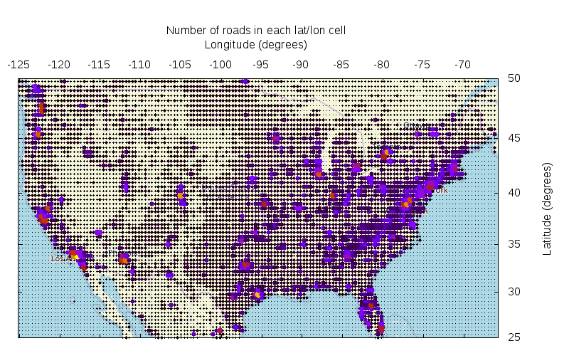
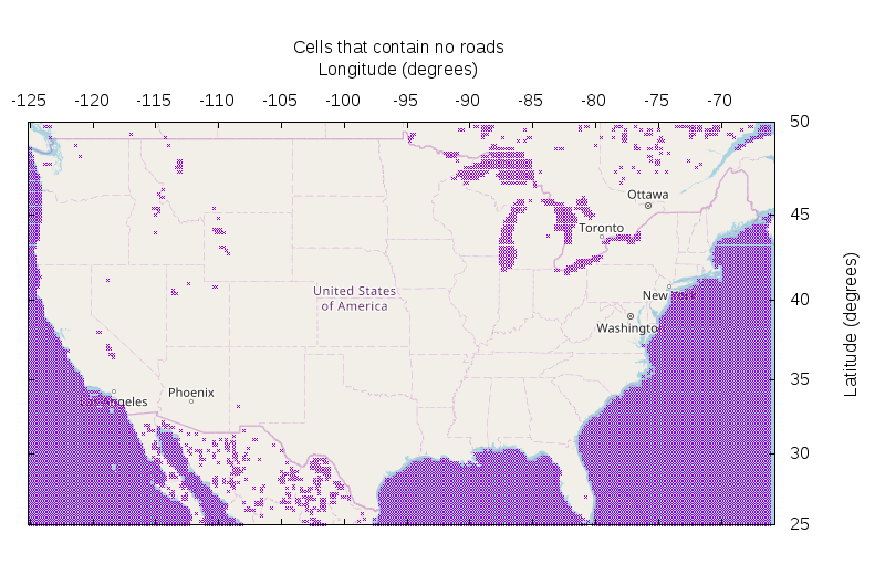
Neat! Here the way counts are represented by bigger points and brighter colors. This plot just exists to look pretty and to tell me that the sampling is functional: road density is correlated with population density. OK. The goal of this was to find empty cells, so let's do that (made with this script):
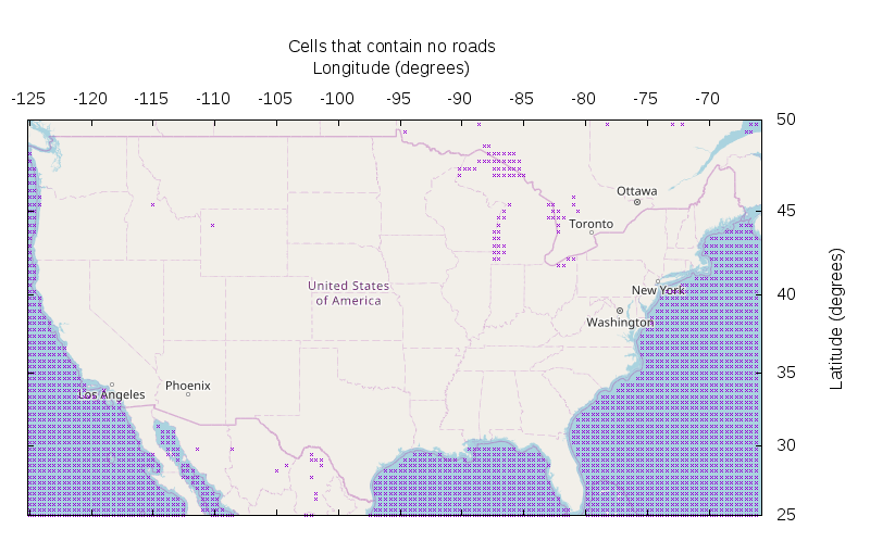
Neat!!! The oceans have no roads. The Great Lakes also have no roads. There's a big roadless chunk on the Mexican side of the Rio Grande, but it looks like that's due more to missing data than to the roadless-ness of that area. So I focus on the US. Looks like there're exactly two empty cells: one in Wyoming (this is the Yellowstone area) and one in Idaho (Frank Church wilderness).
For each of the two candidates I download the actual way data for each of the candidate areas to get a sanity check and to get a bound for the area where I will compute the voronoi diagram. For the Yellowstone area:
$ ./query_rect.sh 43.7 -110.6 44.6 -109.5

$ < query*.json(om[1]) |
    awk '/"lat"/ {lat=$2} /"lon"/ {lon=$2} /}/ {print lon,lat}' |
    sed 's/,//g' |
    feedgnuplot --domain --xlabel lon --ylabel lat --square
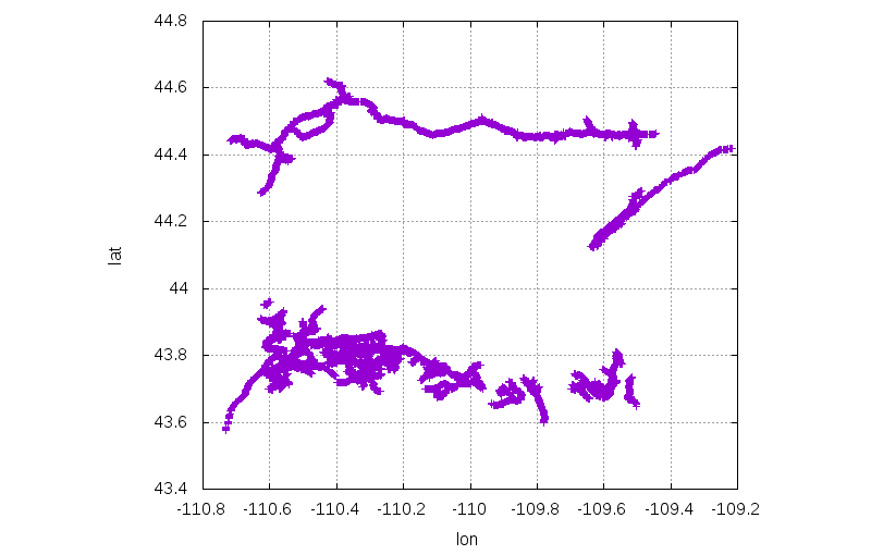
As expected, this looks like an empty area surrounded by roads. Let's process it further, using the previous tools:
$ ../massage_input.pl query*.json(om[1])

$ ../voronoi < $PWD/query*.json(om[1]:s/json/dat/:s/query/points/)
-1936 -481
-4993 34239
-17383 -31726
32848 -2699
distance: 34854.600557

# ../massage_input.pl query*.json(om[1]) -1936 -481 -4993 34239 -17383 -31726 32848 -2699
44.1469937670531,-110.074264145003
44.4600470404567,-110.112910721116
43.8666857606725,-110.266830150028
44.1270516438681,-109.638457792143
Cool! The furthest-out point is 34.85km from the nearest road. We have the coords of this nearest point and of the 3 bounding points that lie on the nearest roads (centers of incident voronoi edges). These look like this:
Doing the same thing for the empty cell in the Frank Church wilderness:
$ ./query_rect.sh 45.1 -115.4 45.7 -114.6

$ < query*.json(om[1]) |
    awk '/"lat"/ {lat=$2} /"lon"/ {lon=$2} /}/ {print lon,lat}' |
    sed 's/,//g' |
    feedgnuplot --domain --xlabel lon --ylabel lat --square
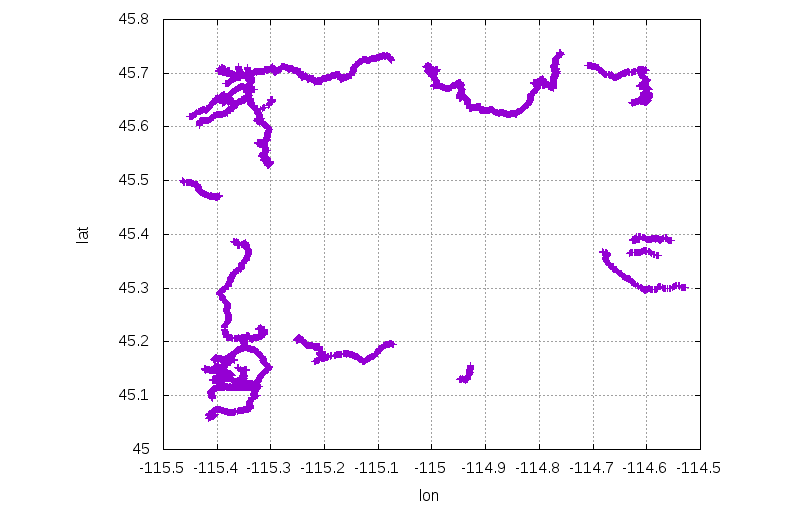
../massage_input.pl query*.json(om[1])

../voronoi < $PWD/query*.json(om[1]:s/json/dat/:s/query/points/)
-1799 2013
5545 25966
-23440 14637
-5850 -22711
distance: 25053.636148

../massage_input.pl query*.json(om[1]) -1799 2013 5545 25966 -23440 14637 -5850 -22711
45.4188043146378,-115.023049362629
45.6347011469176,-114.928683730544
45.5324855876438,-115.300922886895
45.196820550155,-115.074658128517
OK. This area isn't as empty, and you can only get 25.05km away from the nearest road:
So we found a point 34.85km from the nearest road. This is the furthest-out point in areas where we found an empty grid cell. I picked my grid sampling semi-arbitrarily, so now I need to make sure that no circles with a radius larger than 34.85km could lie anywhere else. What is the largest-radius circle that I could possibly fit into areas without empty cells? The worst case is on the Southern edge of my search area (largest distance between adjacent even-latitude divisions). In the worst case I'd have a 2x2 block of cells where the only road points lie in the four opposite corners of this block; these 4 cells would be technically non-empty, but you could fit a large circle there:

My cells are 0.4 degrees per side, so the largest circle that fits among non-empty cells has radius

So in the worst case, we can fit a radius 62.9km circle within my non-empty cells. This is a bit less than double my radius 34.85km circle that I already found. Thus I need to re-run my grid-sampling with a finer grid, and check all the empty areas that turns up. Fine.
The worst case was slighly less than a factor of 2 off. I keep my numbers round, and resample with cell widths of 0.2 degrees instead of 0.4 degrees. This took over 2 hours. Anybody know a better way? The resulting map of empty cells looks like this (data, script):
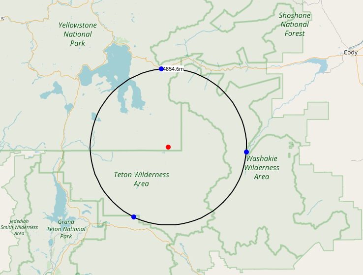
We now have a higher-res view, and there're more locations in the continental US that could contain the point we seek. I checked each one, and that gives a conclusive result. The winner is still the point in Yellowstone National Park computed above: https://caltopo.com/m/T90N with a roadless radius of 34.85km:
There are several noteworthy runners up. In second place, coming in with a roadless radius of 29.0km is the Bob Marshall Wilderness: https://caltopo.com/m/FKP3
In third is the point with a roadless radius of 25.05km that we found above in the Frank Church Wilderness: https://caltopo.com/m/H0TM.
So the original predictions were spot on. I'd like to do this again but staying away from trails also, but that would require even smaller cell sizes, and I really don't want to go through this brute-force grid-search process again. Ideas?